|
Speaker diarization detects which parts of a sound contain speech, and attributes each part to one or more speakers. The output is a list of segments, each segment defined by a start time, an end time and a speaker identifier. Speaker identifiers are natural numbers (1, 2, 3, ...); they are arbitrary labels that roughly follow the order in which the speakers first appear in the sound.
Diarization in Praat always modifies an existing TextGrid by producing one tier per detected speaker. It can be done as part of transcription (so that the transcribed text is split between speaker tiers) or standalone (so that each speaker tier contains the intervals labelled as non-speech or speech). See Speech recognition tutorial for details on how to use it.
Praat performs speaker diarization using a C++/ggml adaptation of pyannote.audio’s pyannote/speaker-diarization-3.1 pipeline. The two neural models used by the pipeline, pyannote/segmentation-3.0 (for segmentation) and wespeaker-voxceleb-resnet34-LM (for speaker embedding, see WeSpeaker), have been converted to ggml format and compiled into Praat, so no external model files are required. The sound is automatically resampled to 16 kHz (the sampling frequency expected by both models) before being processed.
The algorithm is a port of pyannote.audio’s pyannote/speaker-diarization-3.1 pipeline (see Bredin (2023)) with some adaptations. It has four stages.
1. Segmentation. The sound is divided into overlapping 10-second analysis windows. The distance between the starts of two consecutive windows is defined by the Segmentation step (0-1) as a fraction of the window length. For example, a segmentation step of 0.1 makes this distance 1 second, so that consecutive windows have a 90% overlap.
The sound from each analysis window is then sent to the segmentation model, which divides it into 589 frames (each frame spanning approximately 17 milliseconds) and assigns a label to each frame in the following way:
The speaker numbers 1, 2 and 3 are local to each analysis window: speaker 1 in one window is not necessarily the same person as speaker 1 in another. Mapping the window-local speakers to the global ones is the task of stages 2 and 3.
2. Speaker embeddings. The previous stage determined which speaker is active in which frame (for every analysis window). Now, for each window and each speaker active somewhere in it, the frames where this speaker is active are glued together into a single sound, which is then sent to the embedding model. For every such sound, the model produces an embedding: a 256-dimensional vector representing one particular speaker in one particular analysis window. The embeddings of the same speaker (from different analysis windows) tend to be closer to each other than the embeddings of different speakers. This makes the next stage possible.
3. Clustering. The previous stage produces one embedding for each active speaker in each analysis window (so, up to three embeddings per window). The embeddings that are backed by enough non-overlapping speech are considered to be “reliable” and are used in the clustering process; the others are set aside for now.
The reliable embeddings from all analysis windows are first L2-normalized so that they are all located on a 256-dimensional unit hypersphere. They are then grouped using agglomerative hierarchical clustering with centroid linkage. Grouping starts with each embedding forming its own group (with the centre of the group being the embedding itself). At each step, the two groups whose centres are the closest (as measured by Euclidean distance between them) are merged, and the centre of the newly formed group is the mean of all the embeddings in this group. This centre is not L2-normalized, therefore the centres of merged groups lie inside the 256-dimensional hypersphere and become slightly shorter with every merge. This process stops when the distance between the next two closest groups is larger than the Clustering threshold (0-2).
Because the embeddings are L2-normalized, the distance between any two of them lies between 0 (identical) and 2 (opposite), which explains the range of possible values for the clustering threshold.
Each final group represents one speaker; if after reaching the threshold there are still more groups than Max. number of speakers (≥ 2), the merging continues until the resulting number of groups does not exceed that maximum.
Finally, the unreliable embeddings (those not used to form the groups) are attached to their nearest groups. In this way, each window-local speaker is assigned to a global speaker.
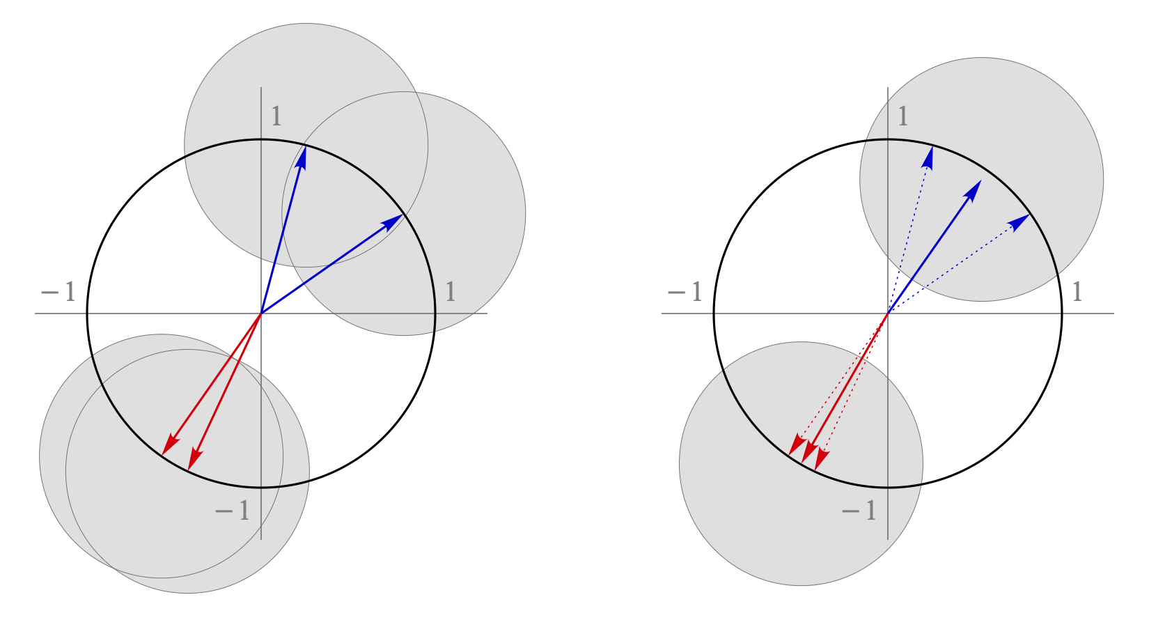
The two figures below show an example of the clustering process for four embeddings in a two-dimensional space. Each group centre is drawn as a solid arrow surrounded by a grey circle whose radius is the clustering threshold (here 0.7, the default). Two groups can be merged only if both their centres lie inside each other’s grey circles (or, in other words, if they are closer than the clustering threshold).
The left figure shows the initial four group centres (the same as the four embeddings). The closest two group centres are drawn in red; these groups are merged first. The next merge involves the groups with the next two closest centres (those drawn in blue). The right figure shows the state after the two merges: the solid arrows are the centres of the two newly formed groups; the dotted arrows are the original embeddings making up each group. Now, neither of the two group centres lies inside the grey circle surrounding the other one. So the two groups are further apart than the clustering threshold; therefore, the clustering process stops, leaving these two groups as the final result.
4. Reconstruction. At stage 1, each analysis window was divided into 589 frames of approximately 17 milliseconds, and each window-frame received a 7-dimensional vector with probabilities of different combinations of local speakers being active. Because the analysis windows overlap, each frame on the global timeline is covered by several windows. The goal of the current stage is to combine the window-frame information across all covering windows, using the local-to-global speaker mapping established at stage 3.
Using the 7-dimensional vectors from stage 1, for each speaker in each window-frame, soft activations are computed, by adding together the probabilities of all combinations in which that speaker is active. This is a number between 0 and 1 (where 0 means definitely silent and 1 means definitely active). These local speakers’ soft activations are then attributed to the global speakers using the mapping from stage 3. After that they are averaged across all the covering windows, to produce an average activation for each global speaker in each global frame.
Separately, the number of simultaneously active speakers in each global frame is found in a similar way. Each window-frame had a winning combination of active speakers (the frame label from stage 1), containing 0, 1 or 2 speakers. For each global frame, this number is averaged across all covering windows, rounded, and capped at 1 when Allow speakers to overlap is off. The resulting number determines how many speakers (those with the highest average activations) are marked active in this frame.
Finally, for each speaker, every uninterrupted sequence of frames in which that speaker is active becomes one segment. The result is a list of segments, where each segment is attributed to one speaker.
For diarization as part of transcription, see transcription with whisper.cpp.
Standalone diarization is available in two ways:
© Anastasia Shchupak 2026-06-01