|
A command available in the Periodicity menu when you select one or more Sound objects. This command autocorrelates the selected Sound object. As a result, a new Sound will appear in the list of objects; this new Sound is the autocorrelation of the original Sound.
The autocorrelation of a continuous time signal f(t) is a function of the lag time τ, and defined as the integral
| Rf (τ) ≡ ∫ f(t) f(t+τ) dt |
If f is a sampled signal (as Sounds are in Praat), with sampling period Δt, the definition is discretized as
| Rf [τ] ≡ ∑t f[t] f[t+τ] Δt |
where τ and t+τ are the discrete times at which f is defined.
The autocorrelation is symmetric: Rf (−τ) = Rf (τ).
You can see in the formula above that if the input Sound is expressed in units of Pa, the resulting Sound should ideally be expressed in Pa2s. Nevertheless, Praat will express it in Pa, because Sounds cannot be expressed otherwise.
This basically means that it is impossible to get the amplitude of the resulting Sound correct for all purposes. For this reason, Praat considers a different definition of autocorrelation as well, namely as the sum
| Rf [τ] ≡ ∑t f[t] g[t+τ] |
The difference between the integral and sum definitions is that in the sum definition the resulting sound is divided by Δt.
The normalized autocorrelation is defined as
| norm-autocorr (f) (τ) ≡ ∫ f(t) f(t+τ) dt / ∫ f2(t) dt |
The boundaries of the integral in 1 are −∞ and +∞. However, f is a Sound object in Praat and therefore has a finite time domain. If f runs from t1 to t2 and is assumed to be zero before t1 and after t2, then the autocorrelation will be zero before t1−t2 and after t2−t1, while between t1−t2 and t2−t1 it is
| Rf (τ) = ∫t1t2 f(t) f(t+τ) dt |
In this formula, the argument of the first f runs from t1 to t2, but the argument of the second f runs from t1+(t1−t2) to t2+(t2−t1), i.e. from t1−(t2−t1) to t2+(t2−t1). This means that the integration is performed over two equal stretches of time during which f must be taken zero, namely a time stretch before t1 and a time stretch after t2, both of duration t2−t1.
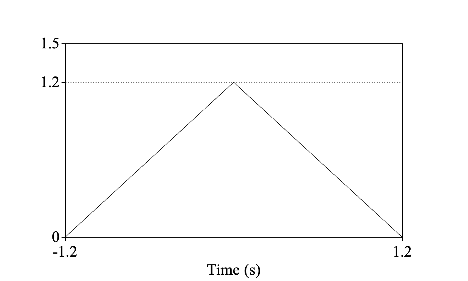
If you consider the sound outside its time domains as similar to what it is within its time domain, instead of zero, the discretized formula in 1 should be based on the average over the jointly defined values of f[τ] and f[t-τ], without counting any multiplications of values outside the time domain. Suppose that f is defined on the time domain [0, 1.2] with the value of 1 everywhere. Its autocorrelation under the assumption that it is zero elsewhere is then
Create Sound from formula: "sound", 1, 0.0, 1.2, 1000, ~ 1
Autocorrelate: "integral", "zero"
Draw: 0, 0, 0.0, 1.5, "yes", "curve"
One mark left: 1.2, "yes", "yes", "yes", ""
but under the assumption that the sound is similar (i.e. 1) elsewhere, its autocorrelation should be
Create Sound from formula: "sound", 1, 0.0, 1.2, 1000, ~ 1
Autocorrelate: "integral", "similar"
Draw: 0, 0, 0.0, 1.5, "yes", "curve"
One mark left: 1.2, "yes", "yes", "yes", ""
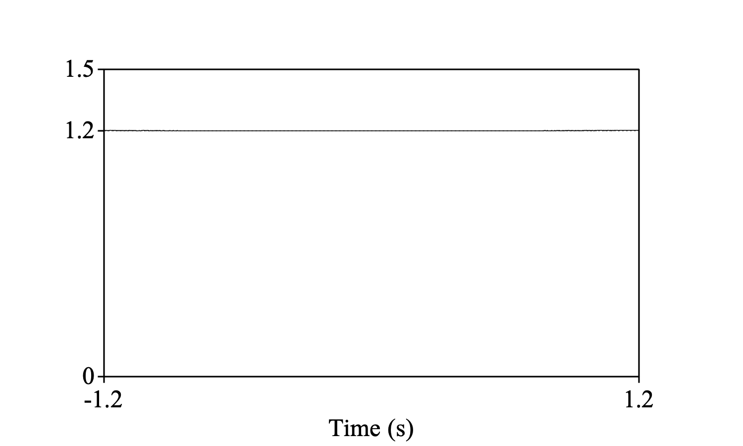
i.e. a constant value of 1.2. This is what you get by choosing the similar option; the autocorrelation will be divided by a triangular function to compensate for the fact that the autocorrelation has been computed over fewer values closer to the edges; this procedure is followed in all autocorrelation-based pitch computations in Praat (see Sound: To Pitch...). For examples, see Boersma (1993).
The start time of the resulting Sound will be the start time of f minus the end time of f, the end time of the resulting Sound will be the end time of f minus the start time of f, the time of the first sample of the resulting Sound will be the first sample of f minus the last sample of f, the time of the last sample of the resulting Sound will be the last sample of f minus the first sample of f, and the number of samples in the resulting Sound will be twice the number of samples of f, minus 1.
If the selected Sound has more than one channel, each channel of the resulting Sound is computed as the cross-correlation of the corresponding channel of the original Sound. For instance, if you autocorrelate a 10-channel sound, the resulting sound will again have 10 channels, and its 9th channel will be the autocorrelation of the 9th channel of the original sound.
The amplitude scaling factor will be the same for all channels, so that the relative amplitude of the channels will be preserved in the resulting sound. For the normalize scaling, for instance, the squared norm of f in the formula above is taken over all channels of f. For the peak 0.99 scaling, the resulting sound will typically have an absolute peak of 0.99 in only one channel, and lower absolute peaks in the other channels.
The autocorrelation is calculated as the cross-correlation of a sound with itself.
© David Weenink & Paul Boersma 2010-04-04,2024