Bayesian Sequential Analysis

• In sequential analysis we don't have a fixed number of observations. Instead, observations come in sequence, and we'd like to decide in favor of $\theta_{0}$ or $\theta_{1}$ as soon as possible. For each $n$ we perform a test: $D(y_{1:n})$. There are three outcomes of $D$:
  • Decide $\theta = \theta_{1}$
  • Decide $\theta = \theta_{0}$
  • Keep testing

• NonBayesian Case Let $T$ be the stopping time of this test. We wish to find an optimal tradeoff between:
  • $P_{FA}$, the probability:: [ $D(y_{1:T}) = 1$, but $\theta = \theta_{0}$]
  • $P_{M}$, the probability: [ $D(y_{1:T}) = 0$, but $\theta = \theta_{1}$]
  • $E_{\theta}(T)$, where $\theta = \theta_0$ or $\theta_1$

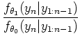
• It turns out, the optimal test again involves monitoring the likelihood ratio. This test is called SPRT for ``Sequential Probability Ratio Test''. It is more insightful to examine this test in the ``log'' domain. The test involves comparing the log likelihood ratio:
  

  $$S_{n} = \frac{f_{\theta_{1}}(y_{1:n})}{f_{\theta_{0}}(y_{1:n})}$$

  
  to positive and negative thresholds $-a < 0$, $b > 0$. The first time $S_{n} < -a$, we stop the test and decide $\theta_{0}$ The first time $S_{n} > b$, we stop and declare $\theta_{1}$. Otherwise we keep on testing.

• There is one ``catch''; in the analysis, we ignore overshoots concerning the threshold boundary. Hence $S_{T} = -a$ or $b$.

• Properties of SPRT The change (first difference) of $S_{n}$ is
  

  $$s_{n} = S_{n} - S_{n-1}$$

  $$= \frac{f_{\theta_{1}}(y_{n} \vert y_{1:n-1})}{f_{\theta_{0}}(y_{n} \vert y_{1:n-1})}$$

  
  For an iid process, we drop the conditioning:
  

  $$s_{n} = \frac{f_{\theta_{1}}(y_{n})}{f_{\theta_{0}}(y_{n})}$$

  
  

  The drift of $S_{n}$ is defined as $E(s_{n} \vert \theta)$. From definitions, it follows that the drifts under $\theta = \theta_{0}$ or $\theta_{1}$ are given by the K-L informations:
  

  $$E(s_{n} \vert \theta_{0}) = -K(\theta_{0}, \theta_{1})$$

  $$E(s_{n} \vert \theta_{1}) = -K(\theta_{1}, \theta_{0})$$

  
  

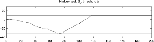
• We can visualize the behavior of $S_{n}$, when in fact $\theta$ undergoes a step transition from $\theta_{0}$ to $\theta_{1}$:

  

• Again, we have practical issues concerning how we choose thresholds $a,b$. By invoking Wald's equation, or some results from martingale theory, these are easily related to the probabilities of error at the stopping time of the test. However, the problem arises how to choose both probabilities of error, since we have a three-way tradeoff with the average run lengths $E_{\theta_{0}}(T)$, $E_{\theta_{1}}(T)$ !!

• Fortunately, the Bayesian formulation comes to our rescue. We can again assign costs to the probabilities of false alarm and miss $C_{FA}, C_{M}$. We also include a cost proportional to the number of observations prior to stopping. Let this cost equal the number of observations, which is $T$. The goal is to minimize expected cost, or sequential Bayes risk. What is our prior information? Again, we must know $P(\theta = \theta_{1}) = \pi_{1}$.

• It turns out that the optimal Bayesian strategy is again a SPRT. This follows from the theory of optimal stopping. Suppose at time $n$, our we have yet to make a decision concerning $\theta$. We must decide among the following alternatives:
  • Stop, and declare $\theta_{0}$ or $\theta_{1}$.
  • Take one more observation.

• We choose to stop only when the minimum additional cost of stopping is less than the minimum expected additional cost of taking one more observation.

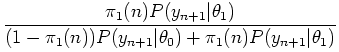
• We compute these costs using the posterior distribution of $\theta$, i.e:
  

  $$\pi_{1}(n) = P(\theta = \theta_{1} \vert y_{1:n})$$

  
  

  which comes by recursively applying Bayes' rule.
  

  $$\pi_{1}(n+1) = \frac{\pi_{1}(n) P(y_{n+1} \vert \theta_{1})}{(1 - \pi_{1}(n)) P(y_{n+1} \vert \theta_{0}) + \pi_{1}(n) P(y_{n+1} \vert \theta_{1})}$$

  $$\pi_{1}(0) = \pi_{1}$$

  
  

• If we stopped after observing $y_{n}$ and declared $\theta = \theta_{0}$, the expected cost due to ``miss'' would be $\pi_{1}(n) C_{M}$. Therefore if we make the decision to stop, the (minimum) additional cost is
  

  $$\rho_{0}(\pi_{1}(n)) = \min \left\{\pi_{1}(n) C_{M}, (1-\pi_{1}(n))C_{FA}\right\}$$

  
  

• The overall minimum cost is:
  

  $$\rho (\pi_{1}(n)) = \min \left\{\rho_{0}(\pi_{1}(n)), 1 + E_{\pi_{1}(n)}[\rho (\pi_{1}(n+1))]\right\}$$

  
  

• In the two-hypothesis case, the implied recursion for the minimum cost can be solved, and the result is a SPRT(!)

• Unfortunately, one cannot get a close form expression for the thresholds in terms of the costs, but the ``Bayes'' formulation allows at least to involve prior information about the hypotheses.

• We will see a much richer extension to the problem of Bayesian change detection.